Training & Monitoring

Training a sparse model has more moving parts than a plain classifier: a learnable pixel budget, a learnable threshold, and quantized bit-widths, each with its own penalty. Our built-in tools make all of it visible so you can see what the model is doing and steer it.

Before you train

Start by looking at the data, so you can pick a sensible starting point for the pixel budget n and the threshold. active_pixels_vs_threshold scans a range of thresholds and reports how many pixels stay active per image (mean, min, max, and a few percentiles):

from sparsepixels.utils import active_pixels_vs_threshold, plot_reduced_examples

active_pixels_vs_threshold(x_train)

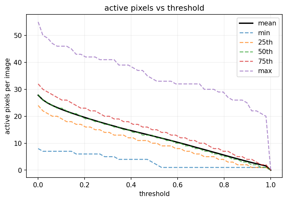
At the threshold you have in mind, read a high percentile or the max to see how many pixels the busiest images carry, and set the initial n a little above that so nothing important is dropped on day one. plot_reduced_examples then shows exactly what a candidate (n, threshold) keeps on a few images, so you can check the digits (or hits) survive:

plot_reduced_examples(x_train, n=20, threshold=0.3, n_examples=3)

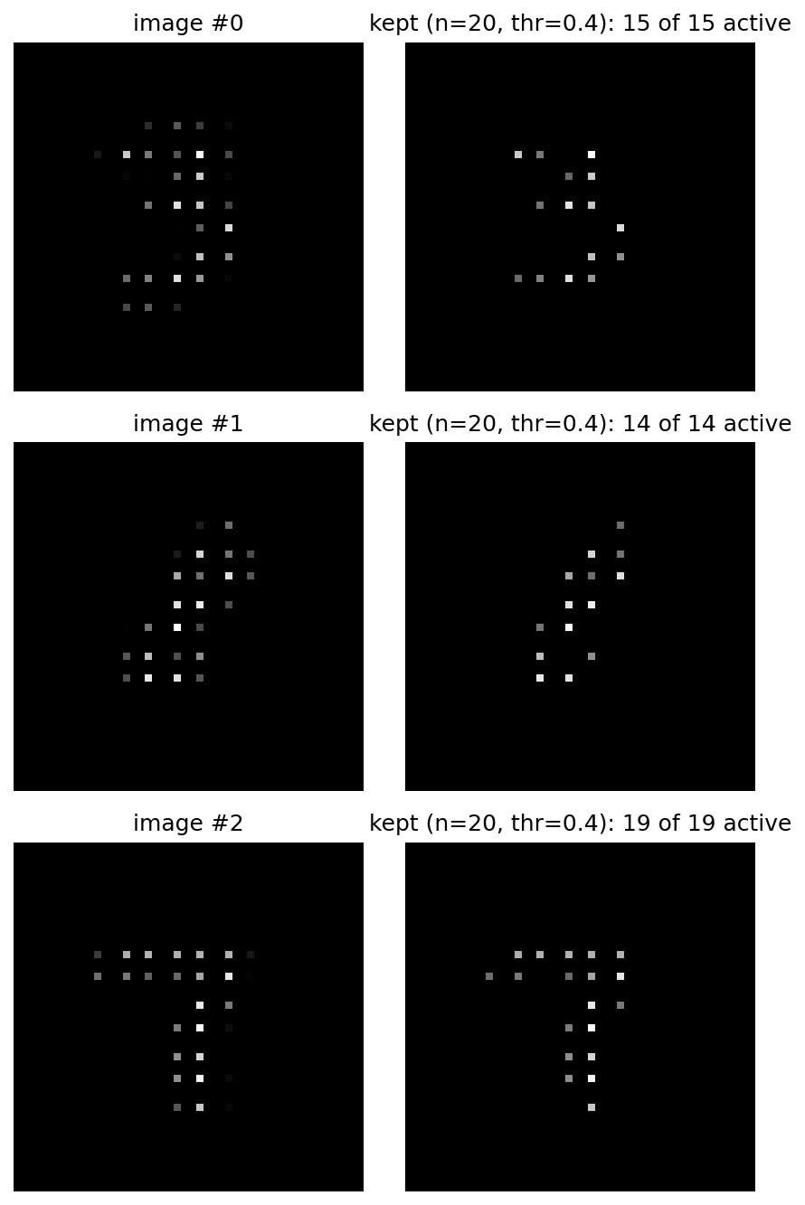
The monitor

Add SparseTrainingMonitor to model.fit's callbacks. Each epoch it records into the history the current budget and threshold of the InputReduce layer (n_max_pixels, threshold), the total ebops, and the loss split into its parts (below). It also applies the sparse EBOPS correction at the start of training, so the reported cost and the regularizer reflect the sparse compute without any manual call.

history = model.fit(..., callbacks=[early_stop, SparseTrainingMonitor()])
plot_history(history, early_stopping=early_stop)

Reading the loss breakdown

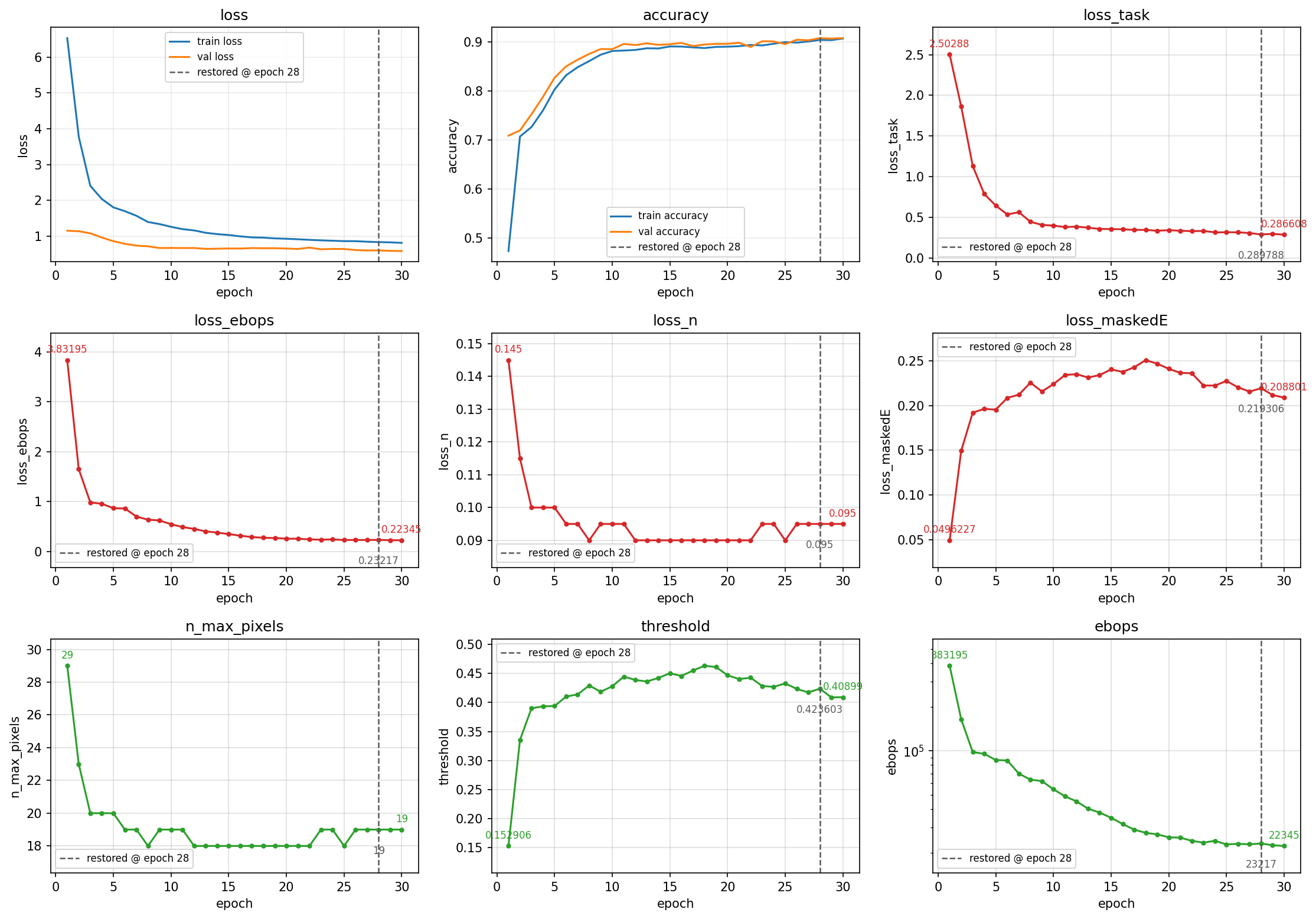
Every penalty is already scaled by its weight, so the parts add up to the total loss:

loss = loss_task + loss_ebops + loss_n + loss_maskedE

Term	What it is
loss_task	the classification (or regression) loss
loss_ebops	the EBOPS regularizer, beta0 * ebops, which shrinks the quantized bit-widths
loss_n	the budget penalty, beta_n * n, which drives the pixel budget down
loss_maskedE	the masked-intensity penalty, which resists throwing away real signal

plot_history draws each of these (in red) next to your metrics, and the sparse diagnostics (n_max_pixels, threshold, ebops, in green), marking the epoch that EarlyStopping restored. A full run from the demo notebook looks like this, with the budget settling and the threshold rising to a stable value:

Tuning the penalties

Three weights set how hard the model is pushed toward cheaper hardware, and they trade against accuracy in different ways:

• beta_n is the price of a kept pixel. Higher beta_n drives the pixel budget n smaller.
• beta_maskedE is the counterweight. It penalizes the fraction of pixel intensity that gets masked, so it pushes back on anything that discards real signal.
• beta0 (set in the LayerConfigScope) is the price of quantization (defined from HGQ2). Higher beta0 shrinks the quantized bit-widths through the EBOPS regularizer: cheaper hardware for a little accuracy.

In practice you are balancing beta_n and beta_maskedE against each other. If the model over-masks, meaning accuracy drops because the threshold climbed too high or n fell too far, lower beta_n or raise beta_maskedE, and start from a larger n or a lower threshold. If it under-masks, meaning it keeps noise and n stays high, do the opposite: raise beta_n or lower beta_maskedE. The data study above gives you the starting n and threshold; the penalties then refine them.

Tip

Change one weight at a time and watch the n_max_pixels, threshold, and validation-accuracy panels in plot_history. A healthy run has the budget and threshold levelling off well before the accuracy starts to suffer.

Quantization summary

After training, inspect the learned bit-widths and per-layer EBOPS:

from sparsepixels.utils import print_quantization, plot_quantization

print_quantization(model)   # per-layer table of weight, bias and activation bit-widths and EBOPS
plot_quantization(model)    # the same as violin plots

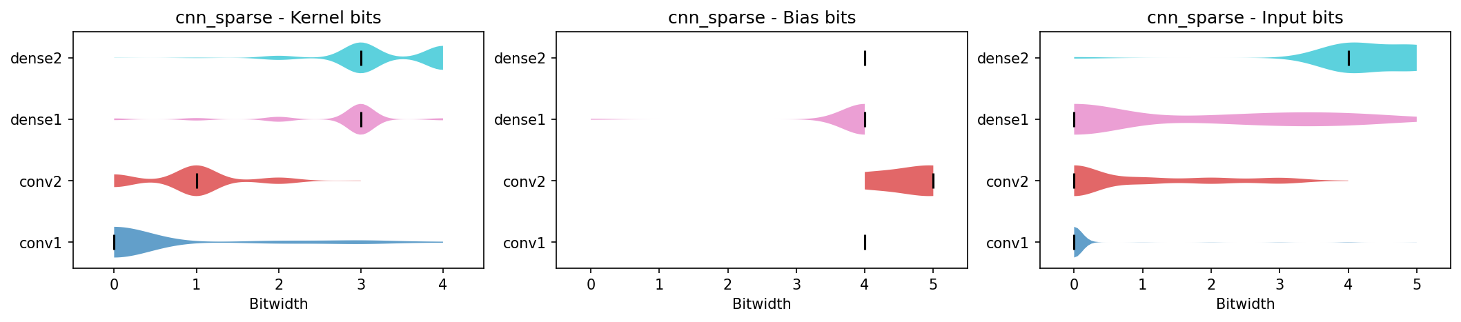
Each violin is one layer. Its horizontal spread is the distribution of learned bit-widths across that layer's kernel, bias, and input values, and the vertical line marks the median. It is a quick way to see where the precision, and therefore the hardware cost, is concentrated.

Deploying the learned values

To retrieve the final pixel budget and threshold after training:

ir = model.get_layer('input_reduce')
n_to_deploy = ir.n_max_pixels     # integer pixel budget
thr_to_deploy = ir.threshold      # activity threshold

The hls4ml converter reads these automatically from the model, so you never pass them by hand. See HLS Conversion.